library(rvest)
library(dplyr)
library(ggplot2)Not long after posting the previous blog post, “Selecting a Literary Corpus from Wikipedia”, I realized there was better way to go about everything. Rather than hard coding the specific Wikipedia pages from which to draw titles, it’s easier to define general years and categories, and then extract from these results. So, in the spirit of the previous blog post, and with the desire to get something out before the end of May, this is a quick addendum and improvement to the methods and process of last time. As always, if you’re allergic to code, feel free to hide it using the button above; alternatively, feel free to skip ahead to the pretty pictures and results at the end.
While the previous blog post resulted in a table of 1,907 titles, this new method yields 13,334.1 In this case, bigger really is better, especially when it comes to understanding an overall picture.
1 Getting started
As before, start by loading necessary packages.
I decided to abstract these functions into a gist available on Github, so the next step is to load it:
devtools::source_gist("https://gist.github.com/jmclawson/79d95f5d10f4e5abd577fc5cf6e8e6ea")With these functions loaded, start by limiting the centuries and national categories to be considered, and then gather the category pages.
centuries <- 16:20
nations <- c("American",
             "Australian",
             "British",
             "Canadian",
             "English",
             "Indian",
             "Irish",
             "New Zealand")

get_cat_pages()
Next, step through the subcategories to collect the URLs to each.
get_subcat_urls()2 Collecting the data
Once the structures are ready, it’s time to check to see if each page exists locally and download it if it doesn’t. As before, this process is mostly to save Wikipedia from what might become a heavy traffic load if we come back to these pages multiple times to glean the data.
This process is contained by the get_subcat_pages() function. It’ll take some time, as it’s designed to wait a randomized length of time to avoid hitting the Wikipedia servers too hard.
get_subcat_pages()With pages stored locally, it’s time to collect and organize the data they contain.
parse_subcat_pages()Once the collecting processes are finished, it’s wise to take a look at the results of things collected. First up is the top part of the table of all novels.
head(corpus_wikipedia)| titles | year | nation | count |
|---|---|---|---|
| Clara Howard | 1801 | American | 2 |
| Equality; or, A History of Lithconia | 1802 | American | 6 |
| Memoirs of Carwin the Biloquist | 1803 | American | 5 |
| Kelroy | 1812 | American | 1 |
| Precaution (novel) | 1820 | American | 2 |
| Owen Chase | 1821 | American | 2 |
Everything looks good there, so there’s no need to modify anything. There were 13,334 titles collected from Wikipedia’s national categories. That’s a lot!
Next, double check the first few rows of novels per nation per year.
head(nation_byyear)| nation | year | count |
|---|---|---|
| American | 1801 | 1 |
| American | 1802 | 1 |
| American | 1803 | 1 |
| American | 1812 | 1 |
| American | 1820 | 1 |
| American | 1821 | 2 |
The full version of this table shows 618 entries summarizing the number of titles represented by each nation for each year. Again, everything looks good and clean.
3 Visualizing the results
After collecting the full list of data, it’s rewarding to see a quantified visualization of the titles collected. In this case, Wikipedia yielded 13,334 titles from these national categories in the range of years in question.
plot_all <- ggplot(corpus_wikipedia, aes(x=year)) +
  geom_bar(aes(fill=nation)) +
  scale_x_continuous(breaks = c(0:12*20+1760)) +
  xlab(NULL) +
  ylab("number of novels") +
  ggtitle("Novels from Anglophonic nations listed on Wikipedia per year") +
  theme_bw()

plot_all
Because the magnitudes of numbers grow wildly out of proportion among the different nations, it’s helpful to drill down into the novels that are not categorized as American or British:
ggplot(corpus_wikipedia[!corpus_wikipedia$nation %in% c("American","British"),]) +
  geom_bar(mapping=aes(x=year, fill=nation)) +
  scale_x_continuous(breaks = c(0:12*20+1760)) +
  xlab(NULL) +
  ylab("number of novels") +
  ggtitle("Non-American, Non-British subset of Wikipedia novels") +
  theme_bw()
Looking at this chart, we notice immediately that some nations are missing. At the beginning of the process, we told our functions that we were interested in the following categories:
nations[1] "American" "Australian" "British" "Canadian" "English"
[6] "Indian" "Irish" "New Zealand"Our final data is lacking in novels in the Wikipedia categories of English, Irish and New Zealand. These omissions come down to inconsistencies in Wikipedia’s category pages, with the category page for New Zealand novels, for instance, lacking years.
We also need to be aware of discrepancies in the novels themselves. While the national categories were chosen to include Anglophonic nations, not all of the novels in the data set will be written in English, as the list of titles of Indian novels suggests.2
head(corpus_wikipedia[corpus_wikipedia$nation=="Indian",])| titles | year | nation | |
|---|---|---|---|
| 13163 | The English Teacher | 1945 | Indian |
| 13164 | All About H. Hatterr | 1948 | Indian |
| 13165 | Randidangazhi | 1948 | Indian |
| 13166 | Sivagamiyin Sapatham | 1948 | Indian |
| 13167 | Vaishali ki Nagarvadhu | 1948 | Indian |
| 13168 | Gunahon Ka Devta (novel) | 1949 | Indian |
Finally, this global corpus allows for a global understanding of some of the trends suggested in the previous corpus, limited to British and American texts.
3.1 World War 1
The smaller set of titles allowed for a consideration only of novels categorized as British and American. A global context should better visualize the impact of World War 1.
ww1 <- ggplot(corpus_wikipedia[corpus_wikipedia$year %in% 1905:1925,],
       aes(x=year)) +
  geom_rect(aes(xmin=1914,xmax=1918.4,ymin=-Inf,ymax=Inf),alpha=0.03,fill="pink") +
  geom_bar() +
  scale_x_continuous(breaks = c(0:9*2+1906)) +
  xlab(NULL) +
  ylab("number of novels") +
  ggtitle("Wikipedia's listing of novels during WW1") +
  theme_bw()

ww1 +
  geom_smooth(data=corpus_byyear[corpus_byyear$year %in% 1905:1925,],
              mapping=aes(y=count,x=year),
              color="red") +
  geom_label(aes(x=1916.2, y=5),
             label="World War I\n7/1914 - 11/1918",
             color="red")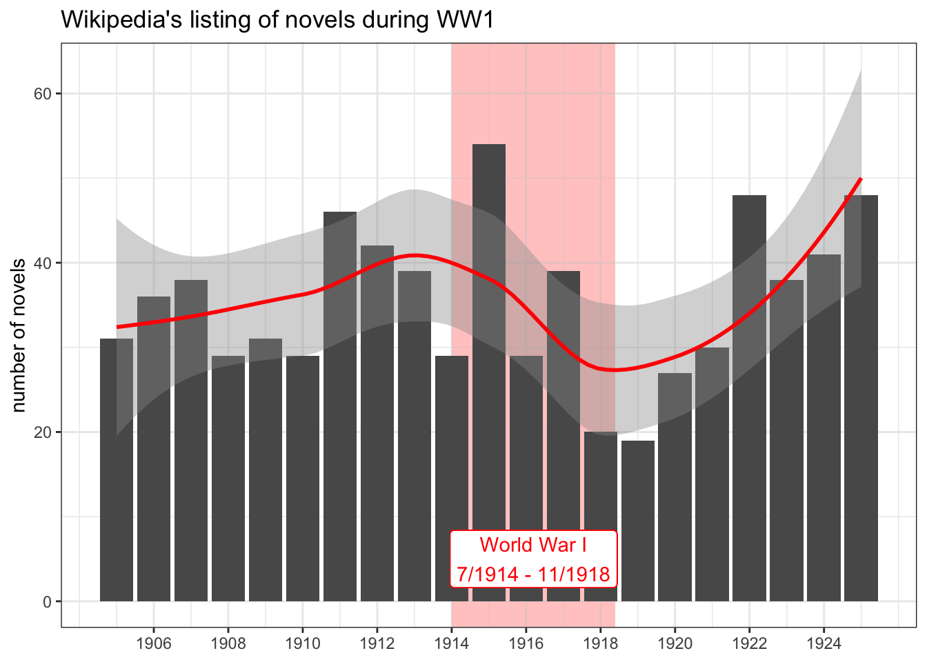
The chart looks very similar to the previous chart including only American and British novels. Breaking it down into constituent parts makes it easy to see why:
ww1 +
  geom_bar(aes(fill=nation)) +
  facet_wrap( ~ nation, ncol=2) +
  scale_x_continuous(breaks = c(0:6*3+1906)) +
  theme_bw() +
  theme(legend.position = "none") +
  ggtitle("Only American and British texts contribute to WW1's downward trend")
It turns out that only American and British texts really contribute to the downward trendline of Wikipedia’s novels listed during World War 1.
3.2 World War 2
Unlike the previous set of titles, this bigger list includes works published through the second world war, too. The data show a similar decline in the listing of wartime novels:
ww2 <- ggplot(corpus_wikipedia[corpus_wikipedia$year %in% 1931:1951,],
       aes(x=year)) +
  geom_rect(aes(xmin=1939,xmax=1945,ymin=-Inf,ymax=Inf),alpha=0.03,fill="pink") +
  geom_bar() +
  scale_x_continuous(breaks = c(0:11*2+1931)) +
  xlab(NULL) +
  ylab("number of novels") +
  ggtitle("Wikipedia's listing of novels during WW2") +
  theme_bw()

ww2 +
  geom_smooth(data=corpus_byyear[corpus_byyear$year %in% 1931:1951,],
              mapping=aes(y=count,x=year),
              color="red") +
  geom_label(aes(x=1942, y=10),
             label="World War 2\n9/1939 - 9/1945",
             color="red")
Breaking it down by national output is only slightly more revealing than the data of World War 1:
ww2 +
  geom_bar(aes(fill=nation)) +
  facet_wrap( ~ nation, ncol=2) +
  scale_x_continuous(breaks = c(0:6*4+1931)) +
  theme_bw() +
  theme(legend.position = "none") +
  ggtitle("Four of the five groups contribute to WW2's downward trend")
Unlike the case in the first world war, the second shows Australian and Canadian texts contributing to the global decline in the numbers of titles listed, albeit in a very minor way when put into the context of American and British works. For understandable reasons, Indian novels aren’t categorized on Wikipedia until 1945.
3.3 International patterns
Having considered the world at war, it may be beneficial to zoom out once again in hopes of making sense of the growth charts for all national literatures. For this comparison, it makes sense to use dissimilar scales among the charts, so that each facet is consistent only within itself; in this way, the trends of national growth—rather than the absolute numbers—can be compared
plot_all +
  facet_wrap( ~ nation, ncol=2, scales="free") +
  ggtitle("National growth charts (inconsistent scales)") +
  theme_bw() +
  theme(legend.position = "none",
        axis.text.x = element_text(angle = 90,
                                         hjust = 1,
                                         vjust=0.5)) +
  ylab(NULL)
Of these, the trend for Canadian novels looks most similar to those of American and British novels, growing mostly consistently over time. On the contrary, Indian novels seem poorly represented on Wikipedia, so it probably doesn’t make sense to make sense out of this chart. Meanwhile, Australian novels show an interesting trend of positive growth until around 1960, with a change in direction until a nadir around 1980. I’m not sure what was happening in Australia at this time, but it would probably warrant further attention.
3.4 Titular words
At the moment, the data frame includes the titles, nation, and publication years from these 13,334 novels. Without the texts themselves, further options for exploration are limited, but it might be fun to peek at trends in the novel titles. After pulling together all the 42,305(!) words from the titles, it’s easy to filter out stop words and find the most common among those that remain:

This cloud of the top 60 words popular in 13,334 titles seems to reveal a lot. Surprisingly, “Oz” and “Conan” make appearances. Otherwise, novelists from this period show a preference for extremes of black and white, of light and dark. Many explore mysteries and themes of death and murder, life and war. And many devote themselves to questions of time, family, the world and humanity. (Or, as is more likely the case, does “man” here reflect a literary fixation on the masculine?)
Finally, comparing the counts of words per title with the publication year shows a greater trend:

Even without a rigorous analysis, the chart shows that, after a slow rise from 1800 until around 1900, the number of words in titles has been on a slight decline since about 1950, especially among British and American texts, and that it’s always been low for Indian novels. At least some of this decline may likely be attributed to the falling out of favor of the double-barrelled Title: or, Subtitle format.
Update: My hunch about subtitles seems incorrect. On one hand, subtitled novels indeed have longer titles. On that same hand, there really is a decline of the prevalence of subtitles, at least within this limited corpus. But juxtaposing title lengths of subtitled and unsubtitled works emphasizes that the trend toward shorter titles is generally followed by novels in both groups:

A larger data set is necessary for testing this kind of a hunch—or even for having it, regardless of how wrong it turns out to be.
4 Conclusions
Wikipedia still isn’t perfect, but it’s a great way to collect a good-sized list of titles. And the methods in this blog post do so more robustly than those in the previous post.
As always, save everything to external files at the end to have a milestone to start back from another time.
saveRDS(corpus_wikipedia,file="corpus_wikipedia.rds")
write.csv(corpus_wikipedia,file="corpus_wikipedia.csv", row.names=FALSE)
My files are available for download here:
Sometime soon, I hope to write up my method for actually getting (some of) these texts, so it’ll be good to be able to start directly from a list of titles.
Footnotes
This data is available for exploration here: jmclawson.net/projects/wiki-corpus.html↩︎
Figuring out which among these are written in English will take time for research beyond the scope of this blog posting.↩︎
Citation
BibTeX citation:
@misc{clawson2019,
  author = {Clawson, James},
  title = {Selecting a {Better} {Corpus}},
  date = {2019-05-30},
  url = {https://jmclawson.net/posts/selecting-a-better-corpus/},
  langid = {en}
}
For attribution, please cite this work as:
Clawson, James. “Selecting a Better Corpus.” jmclawson.net, 30 May 2019, https://jmclawson.net/posts/selecting-a-better-corpus/.