library(tidyverse)
library(tidytext)
library(gutenbergr)1 Getting started
Note
This material was prepared for students in Digital Methods of Literary Text Mining and may be weird outside that context.
As always, we start by loading packages. We’ve been using the tidyverse and tidytext packages from the beginning; this week, we’re also adding gutenbergr, which makes it easy to download books from Project Gutenberg, an online collection of more than 65,000 free books that are out of copyright.
2 An introduction to weighting
By this point, we’re familiar with word frequencies. By counting the number of times a word is used in a document, we can get a sense of how important that word is to that document, relative to other words in the text. And by converting that number to a percentage, we can compare the importance of that word across multiple documents.
One limitation of this approach is that it doesn’t take into consideration words that are common in multiple documents. The word “pie” may be incredibly common in two cookbooks, but there’s a big difference if one book is for desserts and the other is for meat pies. We might focus too much on the common word “pie” and overlook the distinctions between them.
This is why we might add weight to terms that are unusual to each document. We want words like “apple” and “cherry” and “pecan” to jump to the top when we study the cookbook about dessert pies, and we want words like “beef” and “chicken” and “pork” to jump to the top when we look at a cookbook about meat pies.
The technique we use to do this is called “Term frequency–Inverse document frequency” or tf-idf for short.
3 Tf-idf explained
It’s not actually that complicated to understand tf-idf, though our textbook isn’t that clear. We’ll be using a function to do it all, but here’s what it does behind the scenes:
Count the number of times each word is used in one document in a collection.
Divide that number by the total number of words in the document. This converts the number from step 1 into a percentage.
Repeat this for every document in a collection, so each document has a list of words and a list of their percentages.
Count the number of documents each word appears in.
Add a curve to the percentages. Bump up the percentages for words when they’re only used in one document, and bump down the percentage for words that are used in every document. There’s math involved here, but it’s not super important to our class, as long as we get an idea of what it’s doing.
Luckily, one function from the tidytext package will do all that for us.
4 Tf-idf in action
Let’s test it out with some books whose contents we may be familiar with. The gutenbergr package will make it easy to download five scary books. Don’t worry; if scary stories aren’t your thing, we’re not going to read them! These are the five I have in mind:
- Horace Walpole’s The Castle of Otranto (1764)
- Mary Shelly’s Frankenstein (1818)
- Bram Stoker’s Dracula (1897)
- Oscar Wild’s The Picture of Dorian Gray (1890)
- Arthur Conan Doyle’s The Hound of the Baskervilles (1902)
I’ve chosen these because we might know what one or two of them are about. We can use tf-idf to see which words rise to the top and to see what the other books are about.
4.1 Get some books
I’ll start by looking in the gutenberg_metadata table to find the books I’m looking for. I’ll need to look there to find the id number for each book.
gutenberg_metadata |>
  filter(title %in% c("The Castle of Otranto", "Frankenstein; Or, The Modern Prometheus", "Dracula", "The Picture of Dorian Gray", "The Hound of the Baskervilles"))
# A tibble: 18 × 8
gutenberg_id title author gutenberg_author_id language gutenberg_bookshelf
<int> <chr> <chr> <int> <chr> <chr>
1 84 Franken… Shell… 61 en Precursors of Scie…
2 174 The Pic… Wilde… 111 en Gothic Fiction/Mov…
3 345 Dracula Stoke… 190 en Horror/Gothic Fict…
4 696 The Cas… Walpo… 358 en Gothic Fiction
5 2852 The Hou… Doyle… 69 en Detective Fiction/…
6 3070 The Hou… Doyle… 69 en Bestsellers, Ameri…
7 4078 The Pic… Wilde… 111 en Contemporary Revie…
8 6534 Dracula Stoke… 190 en Movie Books/Horror
9 8635 The Hou… Doyle… 69 en Bestsellers, Ameri…
10 9552 The Hou… Doyle… 69 en Bestsellers, Ameri…
11 19797 Dracula Stoke… 190 en Horror/Movie Books
12 20038 Franken… Shell… 61 en Science Fiction by…
13 21520 The Hou… Doyle… 69 en Bestsellers, Ameri…
14 26230 The Pic… Wilde… 111 en <NA>
15 26740 The Pic… Wilde… 111 en <NA>
16 41445 Franken… Shell… 61 en Precursors of Scie…
17 42324 Franken… Shell… 61 en Precursors of Scie…
18 45839 Dracula Stoke… 190 en <NA>
# ℹ 2 more variables: rights <chr>, has_text <lgl>The important column to pay attention to is the one labeled gutenberg_id. Some books have multiple copies, so we’ll limit things by picking the lowest ID number for each book:
gutenberg_metadata |>
  filter(title %in% c("The Castle of Otranto", "Frankenstein; Or, The Modern Prometheus", "Dracula", "The Picture of Dorian Gray", "The Hound of the Baskervilles")) |>
  group_by(title) |>
  summarize(gutenberg_id = min(gutenberg_id))
# A tibble: 5 × 2
title gutenberg_id
<chr> <int>
1 Dracula 345
2 Frankenstein; Or, The Modern Prometheus 84
3 The Castle of Otranto 696
4 The Hound of the Baskervilles 2852
5 The Picture of Dorian Gray 174Next we can download them by their ids. (Run this code chunk only once, so we’re not hitting the Project Gutenberg website too much!)
dracula <- gutenberg_download(345, meta_fields = c("title", "author"))Determining mirror for Project Gutenberg from https://www.gutenberg.org/robot/harvestUsing mirror http://aleph.gutenberg.orgfrankenstein <- gutenberg_download(84, meta_fields = c("title", "author"))
otranto <- gutenberg_download(696, meta_fields = c("title", "author"))
hound <- gutenberg_download(2852, meta_fields = c("title", "author"))
picture <- gutenberg_download(174, meta_fields = c("title", "author"))At this stage, it might be helpful to peak into a book to see what it looks like:
frankenstein# A tibble: 7,357 × 4
gutenberg_id text title author
<int> <chr> <chr> <chr>
1 84 "Frankenstein;" Frankenstein; … Shell…
2 84 "" Frankenstein; … Shell…
3 84 "or, the Modern Prometheus" Frankenstein; … Shell…
4 84 "" Frankenstein; … Shell…
5 84 "by Mary Wollstonecraft (Godwin) Shelley" Frankenstein; … Shell…
6 84 "" Frankenstein; … Shell…
7 84 "" Frankenstein; … Shell…
8 84 " CONTENTS" Frankenstein; … Shell…
9 84 "" Frankenstein; … Shell…
10 84 " Letter 1" Frankenstein; … Shell…
# ℹ 7,347 more rows4.2 Check their most common words
Ultimately, we’re going to join all these books into one big table, from which point we can find the ten most common words in each book:
gothic_books <-
  # use rbind to stick the rows together
  rbind(otranto, frankenstein, dracula, picture, hound) |>
  # convert it to one word per row
  unnest_tokens(word, text) |>
  # drop the gutenberg_id column since we don't need it
  select(-gutenberg_id)

gothic_books |>
  count(title, word) |>
  group_by(title) |>
  arrange(desc(n)) |>
  slice_head(n = 10) |>
  ungroup() |>
  ggplot(aes(x = n, y = reorder(word, n))) +
  geom_col() +
  facet_wrap(vars(title), scales = "free")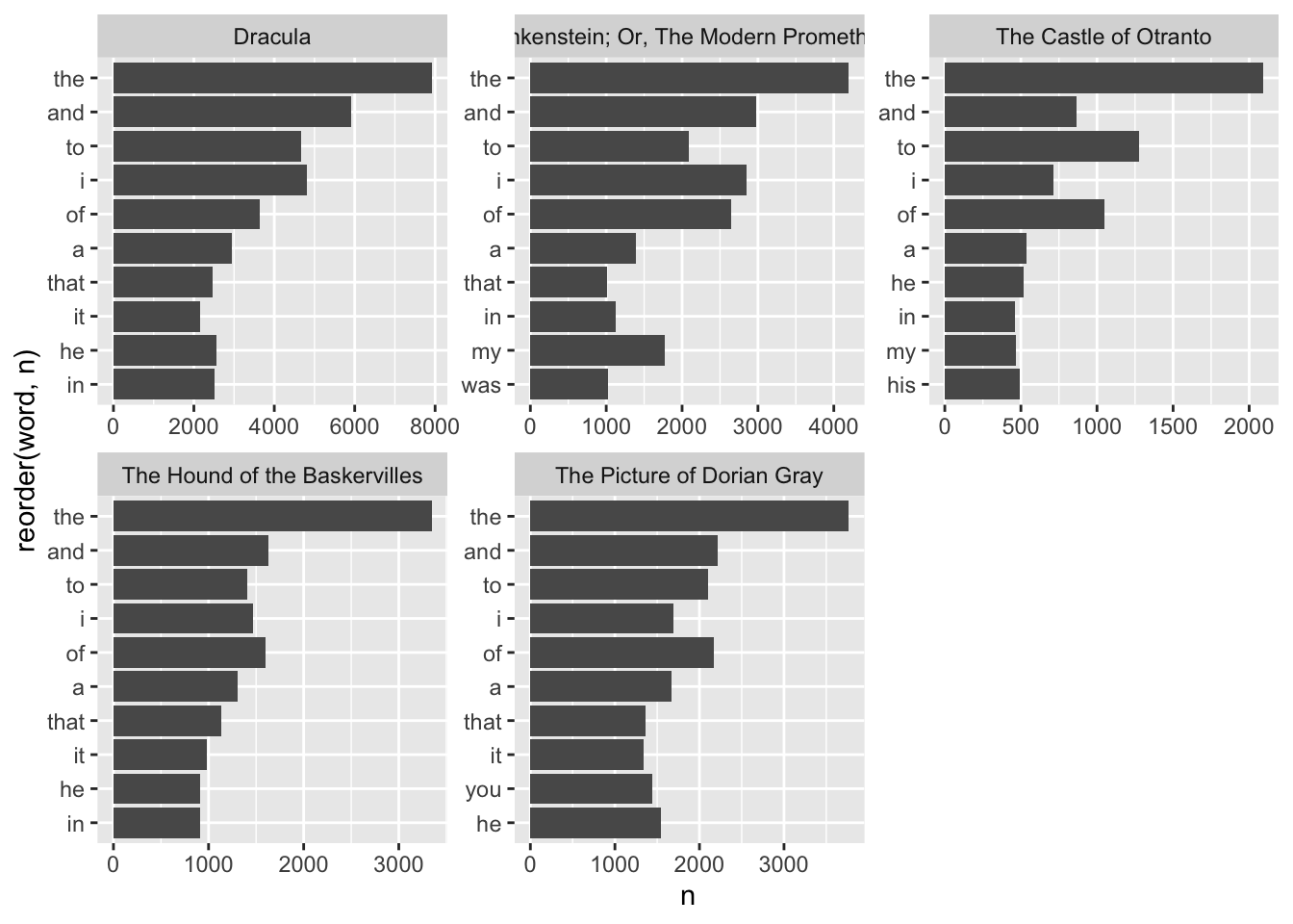
It turns out every book has nearly the same set of words ranking in the top, but none of them is very revealing, if we’re hoping for insight into these books. This is a perfect opportunity for weighting the words that are unique to each book.
5 Convert to tf_idf
Lucky for us, the bind_tf_idf() function handles the dirty work. Let’s take a look at what it shows:
gothic_books_tfidf <- gothic_books |>
  count(title, word) |>
  bind_tf_idf(word, title, n) |>
  arrange(desc(tf_idf))

gothic_books_tfidf
# A tibble: 33,812 × 6
title word n tf idf tf_idf
<chr> <chr> <int> <dbl> <dbl> <dbl>
1 The Castle of Otranto manfred 277 0.00751 1.61 0.0121
2 The Picture of Dorian Gray dorian 410 0.00514 1.61 0.00827
3 The Castle of Otranto matilda 162 0.00439 1.61 0.00707
4 The Castle of Otranto theodore 129 0.00350 1.61 0.00563
5 The Hound of the Baskervilles holmes 187 0.00313 1.61 0.00504
6 The Castle of Otranto hippolita 115 0.00312 1.61 0.00502
7 The Castle of Otranto princess 105 0.00285 1.61 0.00458
8 The Castle of Otranto isabella 180 0.00488 0.916 0.00447
9 The Hound of the Baskervilles moor 165 0.00277 1.61 0.00445
10 The Castle of Otranto thy 143 0.00388 0.916 0.00355
# ℹ 33,802 more rowsHere’s what each step does:
- The
count(title, word)line adds the column callednwhich includes the number of times each word is used in each document, designated by title. - The
bind_tf_idf(word, title, n)line adds the remaining columns fortf(term frequency, or percentage),idf(inverse document frequency, or the portion of our five books that don’t include this word), andtd_idf(term frequency-inverse document frequency, or the combination of these last two values).
We can use that last column to get a better sense of what makes each book stand out from the rest:
gothic_books_tfidf |>
  group_by(title) |>
  arrange(desc(tf_idf)) |>
  slice_head(n = 10) |>
  ungroup() |>
  ggplot(aes(x = tf_idf, y = reorder(word, tf_idf))) +
  geom_col() +
  facet_wrap(vars(title), scales = "free")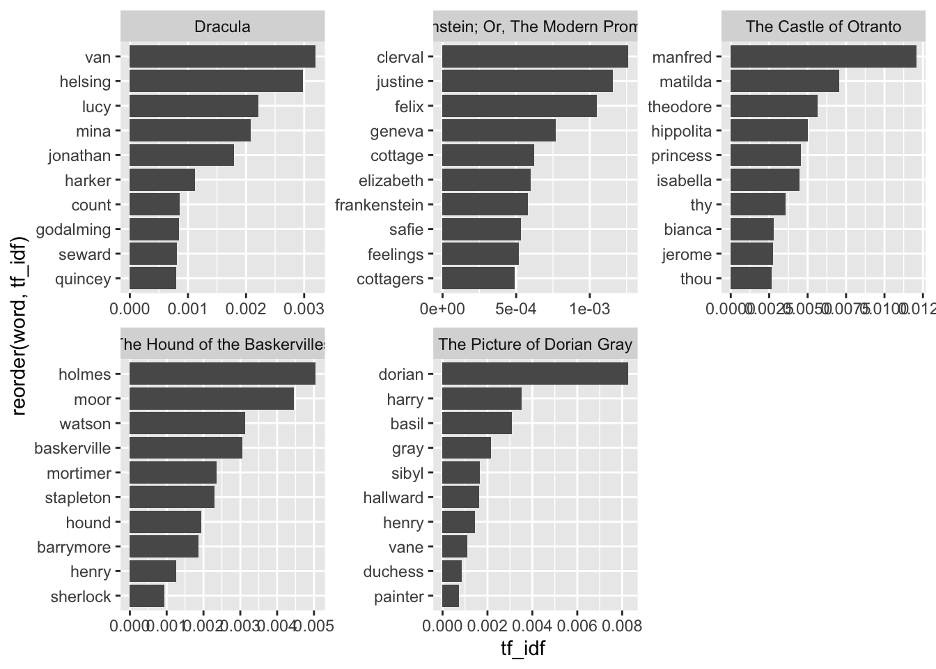
Proper nouns, including place names and character names dominate most of these top words. That makes sense. A book uses its characters’ names a lot, giving each a relatively high frequency, Meanwhile, other books won’t mention these same character names or locations, thereby giving each a high inverse document frequency. When these two high numbers are combined into tf-idf, the result will be even higher.
Hiding within these character names and locations, we can begin to see some important items peaking through. In Frankenstein, we can see mention of “cottage” and “feelings”; anyone who has read the book knows that they’re important in that story. If only we could cut through the proper nouns!
6 Removing proper nouns
One way we can remove words like names and locations is is to drop any words that always start with a capital letter. To do that, we’ll have to back up a bit:
gothic_books_with_caps <-
  # use rbind to stick the rows together
  rbind(otranto, frankenstein, dracula, picture, hound) |>
  # convert it to one word per row, but DON'T convert to lowercase
  unnest_tokens(word, text, to_lower = FALSE) |>
  # drop the gutenberg_id column
  select(-gutenberg_id)
The to_lower = FALSE argument in unnest_tokens() keeps the original character case of words. From here, we can use a filter() to limit the table to words beginning with a lowercase letter, and then use pull() to grab just the “word” column. And we can use a similar step to limit the table to words beginning with an uppercase letter, also using pull() to grab just the one column we need, and unique() cutting out any repeats. In the filter steps below, the ^ character says that we’re looking specifically at the beginning of the word for either a lowercase letter [a-z] or an uppercase letter [A-Z]:
words_starting_lowercase <-
  # start from gothic_books_with_caps, and then
  gothic_books_with_caps |>
  # filter to show only rows where the "word" column starts with a lowercase letter, and then
  filter(str_detect(word, "^[a-z]")) |>
  # grab just the "word" column, and then
  pull(word) |>
  # drop any repeated words
  unique()

words_starting_uppercase <-
  # start from gothic_books_with_caps, and then
  gothic_books_with_caps |>
  # filter to show only rows where the "word" column starts with an UPPERCASE letter, and then
  filter(str_detect(word, "^[A-Z]")) |>
  # convert these to lowercase (so we can compare them later)
  mutate(word = tolower(word)) |>
  # grab just the "word" column, and then
  pull(word) |>
  # drop any repeats
  unique()
Now that we have both lists, we can look for words that are in the second group, words_starting_uppercase, but which never appear in the first group, words_starting_lowercase. This leaves us with words like “Sherlock” and “Holmes” and “Dorian” and “Lucy” and “Geneva” that are proper nouns, always starting with an uppercase letter in these books. The setdiff() function identifies things that are in the first group but not in the second group:
# If a word always begins with a capital letter, save it to a new object called proper_nouns
proper_nouns <- setdiff(words_starting_uppercase, words_starting_lowercase)

length(proper_nouns)
[1] 1452Now I can use this list of 1,472 words to filter my text before graphing my texts:
gothic_books_tfidf |>
  # filter out proper nouns
  filter(!word %in% proper_nouns) |>
  group_by(title) |>
  arrange(desc(tf_idf)) |>
  slice_head(n = 10) |>
  ungroup() |>
  ggplot(aes(x = tf_idf, y = reorder(word, tf_idf))) +
  geom_col() +
  facet_wrap(vars(title), scales = "free")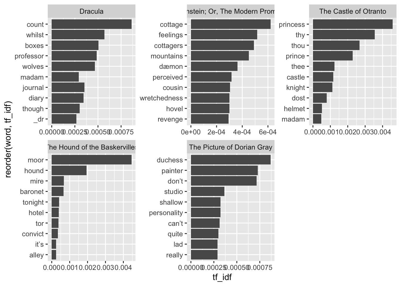
This is much better. Removing the proper nouns is a little tedious, but it allows us to see things more clearly. Here, we can see some themes and plot items beginning to pop out. Additionally—and this was a little unexpected!—we can see that the difference in language is being picked up by the method, too. The older 18th-century book The Castle of Otranto is bubbling up words like “thy” and “thou,” while our late 19th- and early 20th-century books show contractions like “don’t” and “can’t.” We might see if more can be revealed by ignoring these words, too:
gothic_books_tfidf |>
  # filter out proper nouns
  filter(!word %in% proper_nouns) |>
  # filter out archaic words
  filter(!word %in% c("thy", "thou", "thee", "dost", "whilst")) |>
  # filter out any apostrophes to catch contractions, which seem more modern
  filter(!str_detect(word, "'|’")) |>
  group_by(title) |>
  arrange(desc(tf_idf)) |>
  slice_head(n = 10) |>
  ungroup() |>
  ggplot(aes(x = tf_idf, y = reorder(word, tf_idf))) +
  geom_col() +
  facet_wrap(vars(title), scales = "free")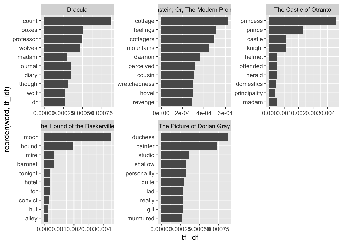
At this point, we’re able to get a pretty good sense of each book’s topic. Dracula is a novel about a count, and there are lots of wolves in it. Frankenstein is largely about revenge in the mountains, inspired by the feelings a “dæmon” developed from watching cottagers. The Castle of Otranto is about royalty, a knight, and (bizarrely) a helmet. The Hound of the Baskervilles does concern a hound out on the moor, or prairie. And The Picture of Dorian Gray is about a shallow lad without much personality, hanging out with a painter in a studio.
We might tidy things up by tweaking a little bit of code:
gothic_books_tfidf |>
  # reorder titles by date
  mutate(
    title =
      factor(title, levels =
               c("The Castle of Otranto",
                 "Frankenstein; Or, The Modern Prometheus",
                 "Dracula",
                 "The Picture of Dorian Gray",
                 "The Hound of the Baskervilles"))) |>
  # filter out proper nouns
  filter(!word %in% proper_nouns) |>
  # filter out archaic words
  filter(!word %in% c("thy", "thou", "thee", "dost", "whilst")) |>
  # filter out apostrophes for contractions and underscores for other weirdnesses
  filter(!str_detect(word, "'|’|_")) |>
  group_by(title) |>
  arrange(desc(tf_idf)) |>
  slice_head(n = 10) |>
  ungroup() |>
  # reorder_within makes sure each book's bars decrease consistently
  ggplot(aes(x = tf_idf, y = reorder_within(word, tf_idf, title))) +
  # add color by filling each column according to its title; don't show a legend
  geom_col(aes(fill = title), show.legend = FALSE) +
  # the labeller here will make the book titles wrap across lines
  facet_wrap(vars(title), scales = "free", labeller = label_wrap_gen()) +
  # we need the next line, since we used reorder_within above
  scale_y_reordered() +
  # changing the theme gets rid of the gray background
  theme_minimal() +
  # the Y-axis label isn't necessary, and the plot title makes the X-axis unneeded, too
  labs(y = NULL,
       x = NULL,
       title = "Top 10 words in each book, ranked by tf-idf",
       subtitle = "Balancing word frequency with corpus frequency reveals distinctive words in each book.") +
  # limit space between bars and word labels
  scale_x_continuous(expand = c(0, 0)) +
  # the next line gets rid of grid lines
  theme(panel.grid = element_blank(),
        # then remove numbers on the X-axis
        axis.text.x = element_blank(),
        # finally, italicize facet labels (book titles)
        strip.text = element_text(face = "italic"))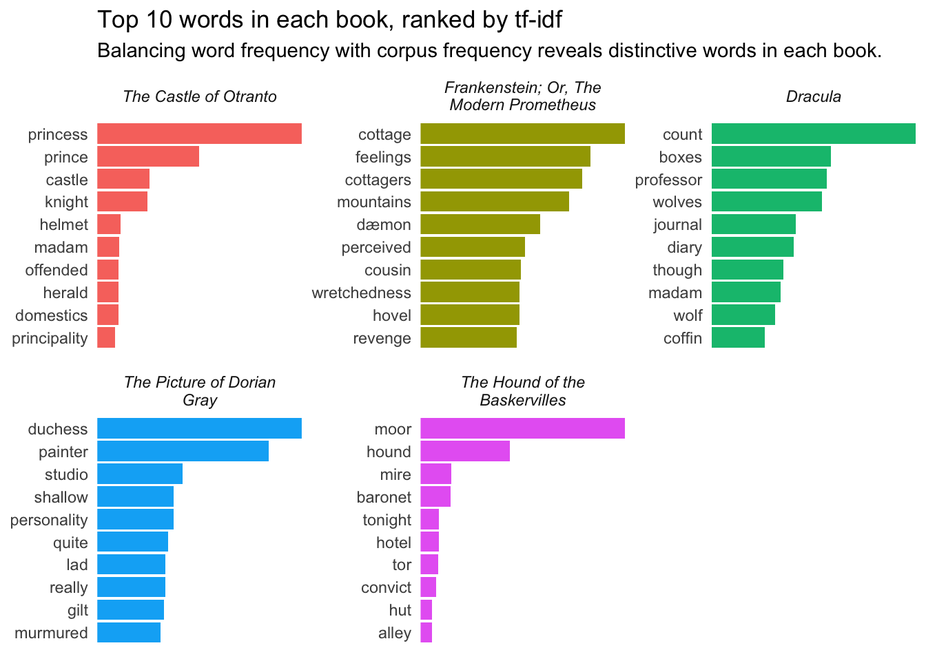
Where you take things from here depends on your creativity and where you’d like to end up. The choices are many, so ask questions!
Citation
BibTeX citation:
@misc{clawson2023,
  author = {Clawson, James},
  title = {Weighted {Word} {Frequencies} with {Tf-idf}},
  date = {2023-03-20},
  url = {https://jmclawson.net/posts/tfidf/},
  langid = {en}
}
For attribution, please cite this work as:
Clawson, James. “Weighted Word Frequencies with Tf-Idf.”
jmclawson.net, 20 Mar. 2023, https://jmclawson.net/posts/tfidf/.