library(tidyverse)1 Intro and Getting Started
Note
This material was prepared for students in Introduction to Data Analytics and may be weird outside that context.
Previously, we used functions from the tidyverse to make sense of a big data set. With select(), we limited columns to those we were most interested in, and with filter() we limited rows to those that fit certain criteria. With mutate(), we modified the data by defining new columns to add, and with group_by() we limited the scope of those definitions to items within a category. By using arrange(), we could change the order of rows in an ascending or descending manner. Finally, with summarize(), we were able to collapse many rows into a single row showing summary statistics. With these tools, we were able to add value to a data set and to gain valuable insight.
We can also add value to a data set by reshaping it and by selectively combining it with other data. In so doing, we’ll find the most value in data that might not already exist in R—and we might find it most useful to export it for some other use when we’re done. For reshaping data, this lesson introduces pivot_longer() and pivot_wider(), which we’ll combine with things we already know for some helpful workflows. For combining data, it introduces left_join() and rbind() for adding columns and rows, respectively. And for importing and exporting data, it introduces read_csv() and write_csv(), which make it possible to bring data into and out of RStudio. Along the way, we’ll be exposed to some additional tricks, including the - (minus sign) notation for column names and functions like rename(), str_remove(), relocate(), and reorder().
Before doing anything, we need to load any packages. We’re keeping it simple by loading the whole tidyverse.
2 Reading a CSV file
So far, we’ve been using data that I’ve provided for you as an R data file, and we’ve been loading it with the load() function. But most of the time, you’ll want to use data you bring into R yourself. For this, we use the read_csv() function. Here, for instance, is how you might load the data set of Louisiana votes, which we looked at in unit two. Notice that this CSV file is saved under the directory called “data”.
votes <- read_csv("data/louisiana_votes.csv")

votes
# A tibble: 64 × 15
state county `Donald Trump` `Joe Biden` `Jo Jorgensen` `Kanye West`
<chr> <chr> <dbl> <dbl> <dbl> <dbl>
1 Louisiana Acadia Pari… 22596 5443 241 45
2 Louisiana Allen Parish 7574 2108 73 15
3 Louisiana Ascension P… 40687 20399 816 134
4 Louisiana Assumption … 7271 3833 68 16
5 Louisiana Avoyelles P… 12028 4979 161 41
6 Louisiana Beauregard … 13575 2542 172 13
7 Louisiana Bienville P… 3891 3067 49 12
8 Louisiana Bossier Par… 38074 15662 632 82
9 Louisiana Caddo Parish 48021 55110 1021 290
10 Louisiana Calcasieu P… 55066 25982 1083 164
# ℹ 54 more rows
# ℹ 9 more variables: `Brian Carroll` <dbl>, `Jade Simmons` <dbl>,
# `Don Blankenship` <dbl>, `President Boddie` <dbl>, `Bill Hammons` <dbl>,
# `Tom Hoefling` <dbl>, `Brock Pierce` <dbl>, `Gloria La Riva` <dbl>,
# `Alyson Kennedy` <dbl>Our data set has 64 rows. Louisiana has 64 parishes, so this isn’t surprising. Since every row shows Louisiana as the state, and since Louisiana’s counties are actually called “parishes,” let’s adjust things a little bit. Although we could add further steps here, referring to the votes object we created in the previous code chunk and then overwriting it with the assignment arrow <-, it’s better practice to go back and edit a code chunk to keep things together; this habit saves you some trouble later when you might accidentally run parts of code out of order. For purposes of this exercise, we’re going to recreate the full workflow in each code chunk so that we can see how things get built up.
We’ll start by dropping the “state” column. The select() function we learned in the previous lesson is most commonly used to choose which columns we want, but it can also be used to name the columns we don’t want if we use a minus sign:
votes <- read_csv("data/louisiana_votes.csv") |>
  select(-state)

votes
# A tibble: 64 × 14
county `Donald Trump` `Joe Biden` `Jo Jorgensen` `Kanye West` `Brian Carroll`
<chr> <dbl> <dbl> <dbl> <dbl> <dbl>
1 Acadi… 22596 5443 241 45 25
2 Allen… 7574 2108 73 15 11
3 Ascen… 40687 20399 816 134 89
4 Assum… 7271 3833 68 16 13
5 Avoye… 12028 4979 161 41 20
6 Beaur… 13575 2542 172 13 18
7 Bienv… 3891 3067 49 12 7
8 Bossi… 38074 15662 632 82 40
9 Caddo… 48021 55110 1021 290 122
10 Calca… 55066 25982 1083 164 89
# ℹ 54 more rows
# ℹ 8 more variables: `Jade Simmons` <dbl>, `Don Blankenship` <dbl>,
# `President Boddie` <dbl>, `Bill Hammons` <dbl>, `Tom Hoefling` <dbl>,
# `Brock Pierce` <dbl>, `Gloria La Riva` <dbl>, `Alyson Kennedy` <dbl>Next, we want to rename “county” to “parish”. We didn’t learn it previously, but dplyr’s rename() function is pretty straightforward:
votes <- read_csv("data/louisiana_votes.csv") |>
  select(-state) |>
  rename(parish = county)

votes
# A tibble: 64 × 14
parish `Donald Trump` `Joe Biden` `Jo Jorgensen` `Kanye West` `Brian Carroll`
<chr> <dbl> <dbl> <dbl> <dbl> <dbl>
1 Acadi… 22596 5443 241 45 25
2 Allen… 7574 2108 73 15 11
3 Ascen… 40687 20399 816 134 89
4 Assum… 7271 3833 68 16 13
5 Avoye… 12028 4979 161 41 20
6 Beaur… 13575 2542 172 13 18
7 Bienv… 3891 3067 49 12 7
8 Bossi… 38074 15662 632 82 40
9 Caddo… 48021 55110 1021 290 122
10 Calca… 55066 25982 1083 164 89
# ℹ 54 more rows
# ℹ 8 more variables: `Jade Simmons` <dbl>, `Don Blankenship` <dbl>,
# `President Boddie` <dbl>, `Bill Hammons` <dbl>, `Tom Hoefling` <dbl>,
# `Brock Pierce` <dbl>, `Gloria La Riva` <dbl>, `Alyson Kennedy` <dbl>Looking great! The only thing bugging me now is that the word “Parish” is added in every line of the column called “parish.” That redundancy isn’t necessary. In the previous lesson, we used the mutate() function to add new columns, but it can also be used to adjust existing columns. With it, we can use str_remove() to remove the string ” Parish” from each row.
Important
I’m removing " Parish", with a leading space, not "Parish". It’s honestly up to you whether you keep the space or remove it, but consistency is easier if you set a rule. To do so, think about how you might later search the data set: If we don’t remove the space, we won’t be able to find the parish called "Lincoln" since our data set would call it "Lincoln " with an extra space at the end.
votes <- read_csv("data/louisiana_votes.csv") |>
  select(-state) |>
  rename(parish = county) |>
  mutate(parish = str_remove(parish, " Parish"))

votes
# A tibble: 64 × 14
parish `Donald Trump` `Joe Biden` `Jo Jorgensen` `Kanye West` `Brian Carroll`
<chr> <dbl> <dbl> <dbl> <dbl> <dbl>
1 Acadia 22596 5443 241 45 25
2 Allen 7574 2108 73 15 11
3 Ascen… 40687 20399 816 134 89
4 Assum… 7271 3833 68 16 13
5 Avoye… 12028 4979 161 41 20
6 Beaur… 13575 2542 172 13 18
7 Bienv… 3891 3067 49 12 7
8 Bossi… 38074 15662 632 82 40
9 Caddo 48021 55110 1021 290 122
10 Calca… 55066 25982 1083 164 89
# ℹ 54 more rows
# ℹ 8 more variables: `Jade Simmons` <dbl>, `Don Blankenship` <dbl>,
# `President Boddie` <dbl>, `Bill Hammons` <dbl>, `Tom Hoefling` <dbl>,
# `Brock Pierce` <dbl>, `Gloria La Riva` <dbl>, `Alyson Kennedy` <dbl>Our data has always been useful, but now it’s also clean and satisfying.
3 Pivoting for summaries
We have a voting breakdown of every parish in Louisiana, which we can use to compare parish political preferences. (Try saying that three times fast!) But we might run into a wall if we try to compare Jo Jorgensen’s 11 votes in tiny Tensas Parish (population 4,043) against the 2,440 votes she earned in East Baton Rouge Parish (population 453,301).1
1 According to U.S. Census estimates for 2021.
Luckily, our data is rich enough that we can calculate how many people voted for the presidential election.
If you remember the mutate() function from the previous lesson—and you should, since we used it in the previous section—your first instinct might be to use it to create a new column called something like “total”, adding up the columns called “Donald Trump” and “Joe Biden” and “Jo Jorgensen” and so on. This is a good instinct. But before you try it, take a look at the next code chunk to see how ungainly it is, adding all these names manually.
votes |>
  mutate(total =
           `Donald Trump` +
           `Joe Biden` +
           `Jo Jorgensen` +
           `Kanye West` +
           `Brian Carroll` +
           `Jade Simmons` +
           `Don Blankenship` +
           `President Boddie` +
           `Bill Hammons` +
           `Tom Hoefling` +
           `Brock Pierce` +
           `Gloria La Riva` +
           `Alyson Kennedy`) |>
  relocate(total, .after = parish)
# A tibble: 64 × 15
parish total `Donald Trump` `Joe Biden` `Jo Jorgensen` `Kanye West`
<chr> <dbl> <dbl> <dbl> <dbl> <dbl>
1 Acadia 28425 22596 5443 241 45
2 Allen 9810 7574 2108 73 15
3 Ascension 62325 40687 20399 816 134
4 Assumption 11235 7271 3833 68 16
5 Avoyelles 17292 12028 4979 161 41
6 Beauregard 16357 13575 2542 172 13
7 Bienville 7050 3891 3067 49 12
8 Bossier 54655 38074 15662 632 82
9 Caddo 104912 48021 55110 1021 290
10 Calcasieu 82663 55066 25982 1083 164
# ℹ 54 more rows
# ℹ 9 more variables: `Brian Carroll` <dbl>, `Jade Simmons` <dbl>,
# `Don Blankenship` <dbl>, `President Boddie` <dbl>, `Bill Hammons` <dbl>,
# `Tom Hoefling` <dbl>, `Brock Pierce` <dbl>, `Gloria La Riva` <dbl>,
# `Alyson Kennedy` <dbl>This definitely works. But it’s ugly because we have to write out each of the 13 candidates’ names—and we can easily imagine the annoyance getting bigger with a larger set of data.
Note
Notice that, when a column name uses special characters like spaces, we have to surround it with back ticks, like this: `column name`.
Tip
This code chunk also shows the previously unmentioned relocate() function, which is useful for moving columns .before or .after other columns. Reording columns isn’t strictly necessary, but it can sometimes be helpful to do so.
More clever is to use pivot_longer() to change the shape of our data from wide to long, and then calculate a total from that.
Let’s focus on Lincoln Parish to understand how this function works.
votes |>
  filter(parish == "Lincoln")
# A tibble: 1 × 14
parish `Donald Trump` `Joe Biden` `Jo Jorgensen` `Kanye West` `Brian Carroll`
<chr> <dbl> <dbl> <dbl> <dbl> <dbl>
1 Lincoln 11311 7559 276 40 27
# ℹ 8 more variables: `Jade Simmons` <dbl>, `Don Blankenship` <dbl>,
# `President Boddie` <dbl>, `Bill Hammons` <dbl>, `Tom Hoefling` <dbl>,
# `Brock Pierce` <dbl>, `Gloria La Riva` <dbl>, `Alyson Kennedy` <dbl>With one row and 14 columns, this table is a clear example of data structured as “wide.” The pivot_longer() function allows us to change the shape from “wide” to “long,” so that we’ll have a limited number of columns (usually three) and a higher number of rows (here, 13 rows, with one for each candidate). The pivot_longer() function expects at least two details:
pivot_longer(data, columns)
The first detail can come from a pipe. The second should list the columns where data can be found. In the example of our Lincoln Parish data, the first column is kind of an identifier. We can use the minus sign trick to say we want to pivot everything except this “parish” column, which we want to keep as a kind of hinge:
votes |>
  filter(parish == "Lincoln") |>
  pivot_longer(-parish)
# A tibble: 13 × 3
parish name value
<chr> <chr> <dbl>
1 Lincoln Donald Trump 11311
2 Lincoln Joe Biden 7559
3 Lincoln Jo Jorgensen 276
4 Lincoln Kanye West 40
5 Lincoln Brian Carroll 27
6 Lincoln Jade Simmons 16
7 Lincoln Don Blankenship 3
8 Lincoln President Boddie 9
9 Lincoln Bill Hammons 11
10 Lincoln Tom Hoefling 9
11 Lincoln Brock Pierce 4
12 Lincoln Gloria La Riva 8
13 Lincoln Alyson Kennedy 2What a change! We now have thirteen rows per parish, with one row for each of the candidates. All of the column names have been moved into a column called “name”, and their values have been moved into a column called “value”. From here, we can use mutate() to add a column that takes the sum of the “value” column:
votes |>
  filter(parish == "Lincoln") |>
  pivot_longer(-parish) |>
  mutate(total = sum(value))
# A tibble: 13 × 4
parish name value total
<chr> <chr> <dbl> <dbl>
1 Lincoln Donald Trump 11311 19275
2 Lincoln Joe Biden 7559 19275
3 Lincoln Jo Jorgensen 276 19275
4 Lincoln Kanye West 40 19275
5 Lincoln Brian Carroll 27 19275
6 Lincoln Jade Simmons 16 19275
7 Lincoln Don Blankenship 3 19275
8 Lincoln President Boddie 9 19275
9 Lincoln Bill Hammons 11 19275
10 Lincoln Tom Hoefling 9 19275
11 Lincoln Brock Pierce 4 19275
12 Lincoln Gloria La Riva 8 19275
13 Lincoln Alyson Kennedy 2 19275From here, one could reshape the data to be wide by using pivot_wider()—the long-lost twin of pivot_longer(). Because we have columns called “name” and “value”, it works without needing any other details inside the parentheses:
votes |>
  filter(parish == "Lincoln") |>
  pivot_longer(-parish) |>
  mutate(total = sum(value)) |>
  pivot_wider()
# A tibble: 1 × 15
parish total `Donald Trump` `Joe Biden` `Jo Jorgensen` `Kanye West`
<chr> <dbl> <dbl> <dbl> <dbl> <dbl>
1 Lincoln 19275 11311 7559 276 40
# ℹ 9 more variables: `Brian Carroll` <dbl>, `Jade Simmons` <dbl>,
# `Don Blankenship` <dbl>, `President Boddie` <dbl>, `Bill Hammons` <dbl>,
# `Tom Hoefling` <dbl>, `Brock Pierce` <dbl>, `Gloria La Riva` <dbl>,
# `Alyson Kennedy` <dbl>But before we do that, let’s apply it to the whole state. Take out the filter() so that we aren’t just looking at Lincoln Parish:
votes |>
  pivot_longer(-parish) |>
  mutate(total = sum(value))
# A tibble: 832 × 4
parish name value total
<chr> <chr> <dbl> <dbl>
1 Acadia Donald Trump 22596 2148062
2 Acadia Joe Biden 5443 2148062
3 Acadia Jo Jorgensen 241 2148062
4 Acadia Kanye West 45 2148062
5 Acadia Brian Carroll 25 2148062
6 Acadia Jade Simmons 18 2148062
7 Acadia Don Blankenship 16 2148062
8 Acadia President Boddie 12 2148062
9 Acadia Bill Hammons 8 2148062
10 Acadia Tom Hoefling 8 2148062
# ℹ 822 more rowsScroll down and check out the value in that “total” column. Oops! Something is definitely wrong. Like last time, we took the sum of the “value” column. But this time, we don’t have 13 rows of data—we have 832! That makes sense because we have 64 parishes, and 13 * 64 = 832.
In other words, we’ve found the total number of presidential votes for the entire state, rather than for each parish. This is a perfect situation for using group_by(). Let’s check out the data in a long format to make sure it does the trick.
votes |>
  pivot_longer(-parish) |>
  group_by(parish) |>
  mutate(total = sum(value))
# A tibble: 832 × 4
# Groups: parish [64]
parish name value total
<chr> <chr> <dbl> <dbl>
1 Acadia Donald Trump 22596 28425
2 Acadia Joe Biden 5443 28425
3 Acadia Jo Jorgensen 241 28425
4 Acadia Kanye West 45 28425
5 Acadia Brian Carroll 25 28425
6 Acadia Jade Simmons 18 28425
7 Acadia Don Blankenship 16 28425
8 Acadia President Boddie 12 28425
9 Acadia Bill Hammons 8 28425
10 Acadia Tom Hoefling 8 28425
# ℹ 822 more rowsThis looks much better! Now we could pivot back to a wider shape, but didn’t we want to compare candidate ratios? We want to see things expressed in a common unit across parishes. The numbers of ballots can be skewed by population size, but the percentages of votes each candidate earned allow us to compare vote distributions regardless of size.
To understand this on a smaller scale, let’s focus on Acadia Parish and Allen Parish, and let’s focus just on Donald Trump’s vote shares, since he carried both parishes. The raw numbers told us that Donald Trump got 15,000 more votes in Acadia Parish and Allen Parish. That’s a lot of people! But adding a “total” column puts this difference in context, as shown in the first table below. Since Acadia Parish had nearly 18,000 more voters in the presidential election, we are left trying to understand the difference in 15,000 votes. How dissimilar was the vote in these two parishes? To answer that question, we’d like to have percentages, as shown in the second table below:
| parish | total | Donald Trump |
|---|---|---|
| Acadia | 28,425 | 22,596 |
| Allen | 9,810 | 7,574 |
| parish | total | Donald Trump |
|---|---|---|
| Acadia | 28,425 | 79.5% |
| Allen | 9,810 | 77.2% |
A 2.3% difference is much more indicative of the difference in voter preference than the huge number 15,000 seems to imply. We find this percentage by pulling out a calculator and dividing the candidate’s votes by the number of total votes. But why not work smarter? Since R can be our calculator, let’s take the opportunity to convert votes from absolute values to a percentage of the vote total. While we’re at it, let’s apply it to the whole data set and save it into a new object with a name that reflects that we’re showing the percentages of votes:
votes_percentages <-
  votes |>
  pivot_longer(-parish) |>
  group_by(parish) |>
  mutate(total = sum(value),
         value = value / total) |>
  pivot_wider()

votes_percentages
# A tibble: 64 × 15
# Groups: parish [64]
parish total `Donald Trump` `Joe Biden` `Jo Jorgensen` `Kanye West`
<chr> <dbl> <dbl> <dbl> <dbl> <dbl>
1 Acadia 28425 0.795 0.191 0.00848 0.00158
2 Allen 9810 0.772 0.215 0.00744 0.00153
3 Ascension 62325 0.653 0.327 0.0131 0.00215
4 Assumption 11235 0.647 0.341 0.00605 0.00142
5 Avoyelles 17292 0.696 0.288 0.00931 0.00237
6 Beauregard 16357 0.830 0.155 0.0105 0.000795
7 Bienville 7050 0.552 0.435 0.00695 0.00170
8 Bossier 54655 0.697 0.287 0.0116 0.00150
9 Caddo 104912 0.458 0.525 0.00973 0.00276
10 Calcasieu 82663 0.666 0.314 0.0131 0.00198
# ℹ 54 more rows
# ℹ 9 more variables: `Brian Carroll` <dbl>, `Jade Simmons` <dbl>,
# `Don Blankenship` <dbl>, `President Boddie` <dbl>, `Bill Hammons` <dbl>,
# `Tom Hoefling` <dbl>, `Brock Pierce` <dbl>, `Gloria La Riva` <dbl>,
# `Alyson Kennedy` <dbl>With these new numbers, we’re able to compare candidates’ performance directly across each parish while accounting for total votes.
4 Joining columns
So far, we’ve been looking at voting in a realistic way. Only the voters who vote get counted. But what if we wanted to compare the vote totals to some other number? For instance, mightn’t it be handy to see what percentage of a parish’s total population voted for a candidate, and what percentage voted in total?
We can use left_join() to add more columns of data to our study. To understand how this might work, let’s first pull in county-by-county population data from the U.S. Census. As before, we’re using read_csv() to read the CSV file as a table in R.
Code
# Helper function to download data if it doesn't already exist locally
get_if_needed <- function(
    url, # Url to be downloaded (necessary)
    filename = NULL, # destination filename (optional)
    destdir = "data" # destination directory (optional)
    ) {

  # If `filename` parameter is not set, it defaults to online file name.
  if(is.null(filename)){
    the_filename <- url |> str_extract("[a-z 0-9 \\- .]+csv")
  } else {
    the_filename <- filename
  }

  # The `destdir` directory will be created if necessary
  if(!dir.exists(destdir)){
    dir.create(destdir)
  }

  filepath <- file.path(destdir, the_filename)

  if(!file.exists(filepath)) {
    download.file(url, destfile = filepath)
  }
}
# Use a helpful function to download this data only once
get_if_needed("https://www2.census.gov/programs-surveys/popest/datasets/2020-2021/counties/totals/co-est2021-alldata.csv")
county_pops <- read_csv("data/co-est2021-alldata.csv")
county_pops# A tibble: 3,194 × 35
SUMLEV REGION DIVISION STATE COUNTY STNAME CTYNAME ESTIMATESBASE2020
<chr> <dbl> <dbl> <chr> <chr> <chr> <chr> <dbl>
1 040 3 6 01 000 Alabama Alabama 5024279
2 050 3 6 01 001 Alabama Autauga County 58805
3 050 3 6 01 003 Alabama Baldwin County 231767
4 050 3 6 01 005 Alabama Barbour County 25223
5 050 3 6 01 007 Alabama Bibb County 22293
6 050 3 6 01 009 Alabama Blount County 59134
7 050 3 6 01 011 Alabama Bullock County 10357
8 050 3 6 01 013 Alabama Butler County 19051
9 050 3 6 01 015 Alabama Calhoun County 116441
10 050 3 6 01 017 Alabama Chambers County 34772
# ℹ 3,184 more rows
# ℹ 27 more variables: POPESTIMATE2020 <dbl>, POPESTIMATE2021 <dbl>,
# NPOPCHG2020 <dbl>, NPOPCHG2021 <dbl>, BIRTHS2020 <dbl>, BIRTHS2021 <dbl>,
# DEATHS2020 <dbl>, DEATHS2021 <dbl>, NATURALCHG2020 <dbl>,
# NATURALCHG2021 <dbl>, INTERNATIONALMIG2020 <dbl>,
# INTERNATIONALMIG2021 <dbl>, DOMESTICMIG2020 <dbl>, DOMESTICMIG2021 <dbl>,
# NETMIG2020 <dbl>, NETMIG2021 <dbl>, RESIDUAL2020 <dbl>, …
Note
The first few lines here are a courtesy to the U.S. Census website. Because we’re downloading a file from there, and since we might collectively run this code many times, we don’t want to keep hitting their server and possibly slow down connections. Those first few lines check to see whether a file exists in our local folder and then downloads it if it doesn’t exist. (Remember, a ! negates any logical test.) In this way, we only visit their website once.
Taking a look at the data shows us that it’s pretty big. We have 3194 rows and 35 columns. Since we don’t care for anything but Louisiana’s data, including just the column for the parish name and the column showing the population estimate for 2020, let’s simplify things:
la_pops <- county_pops |>
  filter(STNAME == "Louisiana") |>
  select(parish = CTYNAME,
         population = POPESTIMATE2020)

la_pops
# A tibble: 65 × 2
parish population
<chr> <dbl>
1 Louisiana 4651203
2 Acadia Parish 57455
3 Allen Parish 22697
4 Ascension Parish 126984
5 Assumption Parish 20968
6 Avoyelles Parish 39616
7 Beauregard Parish 36573
8 Bienville Parish 12899
9 Bossier Parish 128615
10 Caddo Parish 237056
# ℹ 55 more rowsHere, we can see that there’s an unnecessary row for the state as a total. We can remove it, and we can drop “Parish” from each of the parish names. This second step is important because we need to match values in the “parish” column precisely in both data sets.
Important
As before, notice that I’m removing " Parish", including the preceding space, not just "Parish". If you’re not careful about removing that space, then the parish names might not match up when you join data sets. After all, the three strings "Lincoln Parish" and "Lincoln " and "Lincoln" are not equal to each other.
la_pops <-
  county_pops |>
  filter(STNAME == "Louisiana") |>
  select(parish = CTYNAME,
         population = POPESTIMATE2020) |>
  filter(parish != "Louisiana") |>
  mutate(parish = str_remove(parish,
                             " Parish"))

la_pops
# A tibble: 64 × 2
parish population
<chr> <dbl>
1 Acadia 57455
2 Allen 22697
3 Ascension 126984
4 Assumption 20968
5 Avoyelles 39616
6 Beauregard 36573
7 Bienville 12899
8 Bossier 128615
9 Caddo 237056
10 Calcasieu 216416
# ℹ 54 more rowsThings look good, and we’re ready to add the population column to our original data set using left_join(), which expects the following arguments:
left_join(x, y, by)
The x argument is the “left” data set. These are the columns we want to appear first, and they should be the ones that have most of our information in them. The y argument is the “right” data set. Its columns will appear on the right-hand side when we combine things. When we use left_join(), we care about x more than y. Finally, by is where we can define the column names to match between our two data sets. If our data sets have one column that matches in names, then we can skip this part altogether. The message Joining, by = "parish" indicates that the function notices the matching column names and is choosing a by value automatically.
la_votes_population <-
  left_join(votes, la_pops)
Joining with `by = join_by(parish)`la_votes_population# A tibble: 64 × 15
parish `Donald Trump` `Joe Biden` `Jo Jorgensen` `Kanye West` `Brian Carroll`
<chr> <dbl> <dbl> <dbl> <dbl> <dbl>
1 Acadia 22596 5443 241 45 25
2 Allen 7574 2108 73 15 11
3 Ascen… 40687 20399 816 134 89
4 Assum… 7271 3833 68 16 13
5 Avoye… 12028 4979 161 41 20
6 Beaur… 13575 2542 172 13 18
7 Bienv… 3891 3067 49 12 7
8 Bossi… 38074 15662 632 82 40
9 Caddo 48021 55110 1021 290 122
10 Calca… 55066 25982 1083 164 89
# ℹ 54 more rows
# ℹ 9 more variables: `Jade Simmons` <dbl>, `Don Blankenship` <dbl>,
# `President Boddie` <dbl>, `Bill Hammons` <dbl>, `Tom Hoefling` <dbl>,
# `Brock Pierce` <dbl>, `Gloria La Riva` <dbl>, `Alyson Kennedy` <dbl>,
# population <dbl>Our data now shows the population of each parish far to the right. We can combine left_join() with pivot_longer() to recreate our previous table of percentages, only this time calculating the votes each candidate earned as a percentage of a parish’s population.
votes_population <-
  votes |>
  pivot_longer(-parish) |>
  left_join(la_pops) |>
  mutate(value = value/population) |>
  pivot_wider()
Joining with `by = join_by(parish)`votes_population# A tibble: 64 × 15
parish population `Donald Trump` `Joe Biden` `Jo Jorgensen` `Kanye West`
<chr> <dbl> <dbl> <dbl> <dbl> <dbl>
1 Acadia 57455 0.393 0.0947 0.00419 0.000783
2 Allen 22697 0.334 0.0929 0.00322 0.000661
3 Ascension 126984 0.320 0.161 0.00643 0.00106
4 Assumption 20968 0.347 0.183 0.00324 0.000763
5 Avoyelles 39616 0.304 0.126 0.00406 0.00103
6 Beauregard 36573 0.371 0.0695 0.00470 0.000355
7 Bienville 12899 0.302 0.238 0.00380 0.000930
8 Bossier 128615 0.296 0.122 0.00491 0.000638
9 Caddo 237056 0.203 0.232 0.00431 0.00122
10 Calcasieu 216416 0.254 0.120 0.00500 0.000758
# ℹ 54 more rows
# ℹ 9 more variables: `Brian Carroll` <dbl>, `Jade Simmons` <dbl>,
# `Don Blankenship` <dbl>, `President Boddie` <dbl>, `Bill Hammons` <dbl>,
# `Tom Hoefling` <dbl>, `Brock Pierce` <dbl>, `Gloria La Riva` <dbl>,
# `Alyson Kennedy` <dbl>From this data set, we can easily find the number of voters as a percentage of each parish’s population and arrange them by voter turnout:
votes_population |>
  select(-population) |>
  pivot_longer(-parish) |>
  group_by(parish) |>
  summarize(voters = sum(value)) |>
  arrange(desc(voters))
# A tibble: 64 × 2
parish voters
<chr> <dbl>
1 Cameron 0.719
2 St. James 0.626
3 Tensas 0.621
4 Pointe Coupee 0.598
5 St. Helena 0.566
6 Iberville 0.556
7 De Soto 0.549
8 Catahoula 0.548
9 Bienville 0.547
10 St. Charles 0.543
# ℹ 54 more rowsImpressive turnout, Cameron Parish! Way to get out the vote!
5 Binding rows
In looking through data like this, you might realize that there are rows missing. Say, for instance, a couple parishes haven’t yet finished voting. When those votes come in, they’ll probably be reported in tables that look similar to the one we already have, though their columns might be ordered by vote share.
Code
# function to create a fictional parish randomized by data in the set
fictional_parish <- function(df, imaginary) {
  random_column_order <-
    colnames(df)[2:ncol(df)] |>
    sample(ncol(df)-1)

  random_numbers <- df[,2:ncol(df)] |>
    as.matrix() |>
    sample(ncol(df)-1) |>
    setNames(random_column_order) |>
    sort(decreasing = TRUE)

  data.frame(parish = imaginary,
             value = random_numbers) |>
    rownames_to_column(var = "name") |>
    pivot_wider()
}

# create two fictional parishes
votes_chinquapin <- fictional_parish(votes, "Chinquapin")
votes_renard <- fictional_parish(votes, "Renard")
Data from these parishes might look like this:
votes_chinquapin# A tibble: 1 × 14
parish `President Boddie` `Alyson Kennedy` `Jo Jorgensen` `Jade Simmons`
<chr> <dbl> <dbl> <dbl> <dbl>
1 Chinquapin 38074 7538 2108 55
# ℹ 9 more variables: `Brian Carroll` <dbl>, `Don Blankenship` <dbl>,
# `Donald Trump` <dbl>, `Joe Biden` <dbl>, `Tom Hoefling` <dbl>,
# `Bill Hammons` <dbl>, `Kanye West` <dbl>, `Brock Pierce` <dbl>,
# `Gloria La Riva` <dbl>votes_renard# A tibble: 1 × 14
parish `Brian Carroll` `President Boddie` `Donald Trump` `Joe Biden`
<chr> <dbl> <dbl> <dbl> <dbl>
1 Renard 55066 39 30 13
# ℹ 9 more variables: `Alyson Kennedy` <dbl>, `Kanye West` <dbl>,
# `Brock Pierce` <dbl>, `Don Blankenship` <dbl>, `Jo Jorgensen` <dbl>,
# `Gloria La Riva` <dbl>, `Tom Hoefling` <dbl>, `Bill Hammons` <dbl>,
# `Jade Simmons` <dbl>Wouldn’t it be nice to combine these tables with our original voter data? The rbind() function makes it easy to add rows in this way, as long as we have matching column names in whatever order:
updated_votes <-
  rbind(votes,
        votes_chinquapin,
        votes_renard)

updated_votes
# A tibble: 66 × 14
parish `Donald Trump` `Joe Biden` `Jo Jorgensen` `Kanye West` `Brian Carroll`
<chr> <dbl> <dbl> <dbl> <dbl> <dbl>
1 Acadia 22596 5443 241 45 25
2 Allen 7574 2108 73 15 11
3 Ascen… 40687 20399 816 134 89
4 Assum… 7271 3833 68 16 13
5 Avoye… 12028 4979 161 41 20
6 Beaur… 13575 2542 172 13 18
7 Bienv… 3891 3067 49 12 7
8 Bossi… 38074 15662 632 82 40
9 Caddo 48021 55110 1021 290 122
10 Calca… 55066 25982 1083 164 89
# ℹ 56 more rows
# ℹ 8 more variables: `Jade Simmons` <dbl>, `Don Blankenship` <dbl>,
# `President Boddie` <dbl>, `Bill Hammons` <dbl>, `Tom Hoefling` <dbl>,
# `Brock Pierce` <dbl>, `Gloria La Riva` <dbl>, `Alyson Kennedy` <dbl>Our new parishes are added at the very bottom of the chart. We could either page through to get to see them, or we could use the tail() function to show the last few rows:
tail(updated_votes)# A tibble: 6 × 14
parish `Donald Trump` `Joe Biden` `Jo Jorgensen` `Kanye West` `Brian Carroll`
<chr> <dbl> <dbl> <dbl> <dbl> <dbl>
1 West B… 7684 6200 122 42 10
2 West C… 4317 710 12 3 3
3 West F… 3863 2298 66 15 6
4 Winn 4619 1543 36 4 3
5 Chinqu… 18 6 2108 3 33
6 Renard 30 13 4 10 55066
# ℹ 8 more variables: `Jade Simmons` <dbl>, `Don Blankenship` <dbl>,
# `President Boddie` <dbl>, `Bill Hammons` <dbl>, `Tom Hoefling` <dbl>,
# `Brock Pierce` <dbl>, `Gloria La Riva` <dbl>, `Alyson Kennedy` <dbl>Even though columns were ordered differently in our two data sets, they were matched perfectly by their names. The first data set determined the order of columns in the result, and its rows come on top.
6 Writing a CSV file
Lastly, we can export data in much the same way that we imported it:
write_csv(updated_votes,
          file = "data/louisiana_votes_updated.csv")
In this way, you can later use your CSV file in other tools, like ArcGIS.
7 Plotting the results
Now that our data uses percentage to show a common unit across all parishes, we can make a simple bar chart to visualize a candidate’s vote share in each parish. Here, for instance, is a bar chart of Jo Jorgensen’s vote share in each of the parishes:
votes_percentages |>
  ggplot(aes(y = parish,
             x = `Jo Jorgensen`)) +
  geom_col()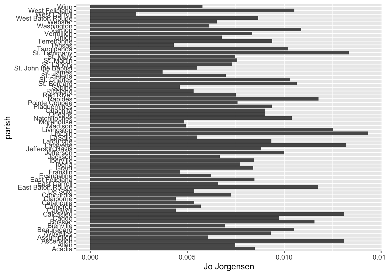
The parish names on the left are in alphabetical order starting at the bottom going up. We can reorder these pretty easily with the reorder() function. Here, we’re reording strings in the the parish column by values in the Jo Jorgensen column:
votes_percentages |>
  ggplot(aes(y = reorder(parish, `Jo Jorgensen`),
             x = `Jo Jorgensen`)) +
  geom_col()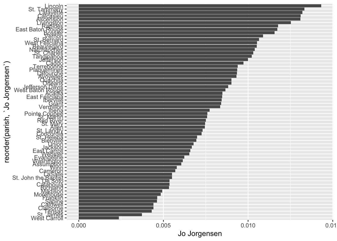
Check out Lincoln Parish! Since we know the total number of votes in each parish, we can also color the bars by parish size. Who knows—it might reveal some trend.
votes_percentages |>
  ggplot(aes(y = reorder(parish, `Jo Jorgensen`),
             x = `Jo Jorgensen`,
             fill = total)) +
  geom_col()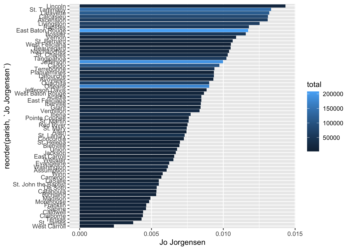
I guess it’s kind of revealing that the parishes where Jorgensen earned the lowest share of votes tended to be smaller parishes, where fewer than 100,000 votes were cast. Lincoln Parish is a clear outlier. We’ll keep this coloring.
In the final step, we’re going to add a little polish to the chart by adjusting the labels and theme and by making the chart a little taller.
Code
#| fig-height: 7
  # Adding fig-height or fig-width to the top of a code
  # chunk lets you adjust the output size of a figure
  # resulting from ggplot. You'll have to play around
  # with numbers to find something you like.

votes_percentages |>
  ggplot(aes(y = reorder(parish, `Jo Jorgensen`),
             x = `Jo Jorgensen`,
             fill = total)) +
  geom_col() +

  # scale_x_continuous() lets me adjust the x-axis. Within
  # it, "labels" lets me format the number of the axis
  # labels. The scales package offers handy functions for
  # formatting different kinds of numbers. On the next line,
  # setting "expand" to 0 lets me shrink the gap between
  # labels and bars.
  scale_x_continuous(
    labels = scales::label_percent(),
    expand = c(0,0)) +

  # scale_fill_continuous() lets me adjust the legend of a
  # "fill" aesthetic. Within it, "labels" lets me format the
  # numbers used in the legend, and the scales package helps
  # in formatting the numbers to look better.
  scale_fill_continuous(
    labels = scales::label_comma()) +

  # labs() lets me set certain labels for key parts of the
  # plot. Arguments y and x let me set the y-axis and x-axis
  # labels, while fill lets me rename the title of the
  # "fill" legend.
  labs(
    y = "Parish",
    x = "Jo Jorgensen's share of the vote",
    fill = "Total votes cast \nin each parish") +

  # I'm not a big fan of that default gray background, and
  # theme_minimal() lets me make it white.
  theme_minimal() +

  # Finally, I don't need the horizontal grid lines in the
  # background, so I'm removing them.
  theme(panel.grid.major.y = element_blank(),
        panel.grid.minor.y = element_blank())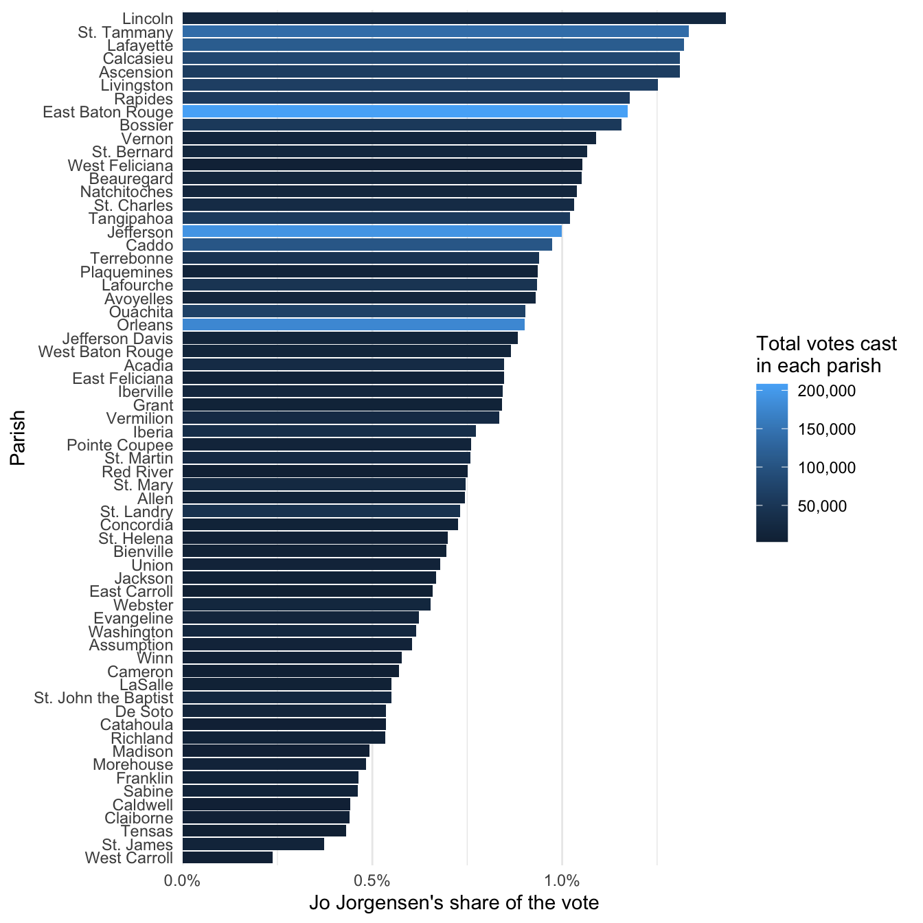
Citation
BibTeX citation:
@misc{clawson2022,
  author = {Clawson, James},
  title = {Importing, {Pivoting,} and {Combining} {Data} {Sets}},
  date = {2022-11-02},
  url = {https://jmclawson.net/posts/import-pivot-join/},
  langid = {en}
}
For attribution, please cite this work as:
Clawson, James. “Importing, Pivoting, and Combining Data
Sets.” jmclawson.net, 2 Nov.
2022, https://jmclawson.net/posts/import-pivot-join/.